Methodology

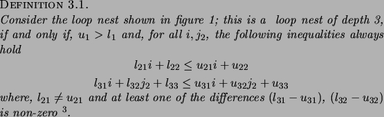
A subclass of the loop nests shown in figure 1 is defined as follows:

³

Definition 3.1 provides the basis for the following theorem.

Figure 2: An example of a canonical loop nest of depth 3.

       DOALL I=1,N
          DO J=3,2*I+1
             DO K=J+2,5*I
                (statements)
             ENDDO
          ENDDO
       ENDDO

 
In order to illustrate the results of Theorem 3.1, consider the loop nest shown in figure 2. Assuming that N $>$ 1, then the inequalities 3 $\leq$ 2*I+1 and J+2 $\leq$ 5*I always hold, while, for each inequality, the coefficients of I are non-zero; hence, the requirements of Definition 3.1 are satisfied and the loop nest is a canonical loop nest of depth 3. Based on Theorem 3.1 and assuming that the number of iterations of the outer loop, N, is a multiple of $2p^2$, where $p$ is the number of processors, partitioning the loop nest according to (4) leads to perfect load balance.

Figure: Geometrical representation of the loop nest shown in FIG. .

To provide an intuitive view of this partitioning scheme, the corresponding geometrical representation of the original loop nest is shown in figure 3.a. Assuming that two processors are used, the index of the outer loop is partitioned into 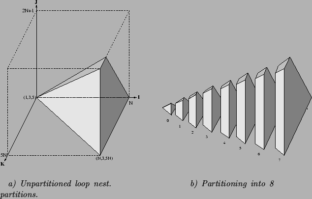$2 \cdot 2^2 = 8$ partitions; the corresponding polytope for each partition is shown in figure 3.b. Then, applying (4), the first processor is assigned partitions 0, 3, 5, and 6, while the second processor is assigned partitions 1, 2, 4, and 7; in geometrical terms, the polytopes have been assigned to two groups in such a way that the total volume of the polytopes in each group is the same.

 
The partitioning technique suggested in the proof of Theorem 3.1 can also be applied when the number of iterations of the outer loop, $n$, is not a multiple of $2p^2$; in this case, assuming that partitioning along the index of the outermost loop is performed as evenly as possible (that is, each partition has a number of iterations which differs by at most 1 from that of any other partition), a small value of load imbalance is expected. Theorem 3.1 can also be extended to cover cases where there are more than one inner loops at the same level (i.e., loops which are surrounded only by the same outer loops) whose bounds depend on the index of a surrounding loop; the necessary requirement is that, for any loop, the lower bound is always less than or equal to the upper bound. Finally, in the general case, where not all the inequalities in Definition 3.1 hold, index set splitting can be applied to transform the original loop nest into multiple adjacent loop nests, each of which satisfies the requirements of Definition 3.1 [12].