In order to illustrate the above, consider again Sweep3D
(which was mentioned in the Introduction) [13]
The main body of the code, that is the subroutine sweep(),
consists of a wavefront computation
on a 3-dimensional grid of cells.
The subroutine computes the flux of neutron particles through each cell
along several possible directions (discretized angles) of travel.
The angles are grouped into 8 octants corresponding to the 8 diagonals
of the cube.
Along each angular direction,
the flux of each interior cell depends on the fluxes
of three neighboring cells. This corresponds to a
3-dimensional pipeline for each angle, with parallelism existing
between angles within a single octant.
The current version of the code partitions the ![]() and
and ![]() dimensions
of the domain among the processors.
To improve the balance between parallel utilization and communication
in the pipelines, the code blocks the third (
dimensions
of the domain among the processors.
To improve the balance between parallel utilization and communication
in the pipelines, the code blocks the third (![]() ) dimension and also
uses blocks of angles within each octant.
) dimension and also
uses blocks of angles within each octant.
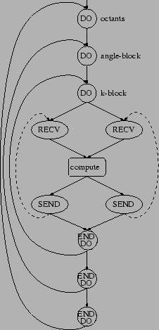
The static task graph for the main body of the code is shown in Figure 1(a). Each node of the graph represents a different task node, where circles correspond to control flow operations, ellipses to communication operations, and rectangles to computation (each rectangle represents a condensed task node, viz., a task node in the static task graph that will be instantiated into several instances of condensed tasks in the condensed dynamic task graph). Solid lines denote those precedence edges of the task graph that are enforced implicitly by intraprocessor control flow while the dotted lines denote those that require interprocessor communication.1The program uses blocking communication operations (MPI_Send and MPI_Recv), each of which is represented by a single communication task.
|
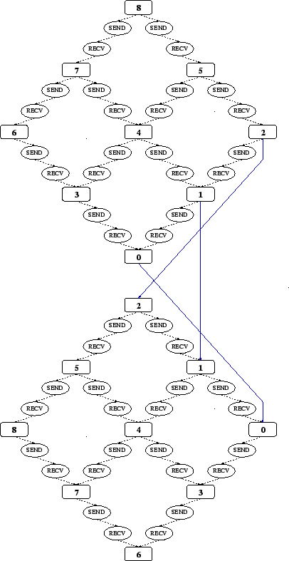
Figure 1(b) shows part of the condensed dynamic task
graph on a ![]() processor grid (recall that loops are
fully unrolled in the dynamic task graph).
The graph corresponds to the last wavefront of octant 2 (top) and the
first wavefront of octant 3 (bottom).
The number inside each computation task
corresponds to the processor executing that task.
processor grid (recall that loops are
fully unrolled in the dynamic task graph).
The graph corresponds to the last wavefront of octant 2 (top) and the
first wavefront of octant 3 (bottom).
The number inside each computation task
corresponds to the processor executing that task.
Using the condensed form of the dynamic task graph described
earlier (see Section 3.4), the size
of the dynamic task graph can be kept reasonable. Thus, for the
the subroutine sweep() with a ![]() problem size on a
problem size on a
![]() processor grid, the dynamic task graph would contain over
processor grid, the dynamic task graph would contain over
![]() tasks, whereas the
condensed dynamic task graph has only 3570 tasks.
tasks, whereas the
condensed dynamic task graph has only 3570 tasks.