MU0 - a simple computer

MU0 - a simple computer

The essence of a computer can be captured in some very simple properties:

• information in memory
• manipulation of information by programs
• decision making on the basis of stored information

A simple view of MU0 considers it as having just 2 components and a link between them:

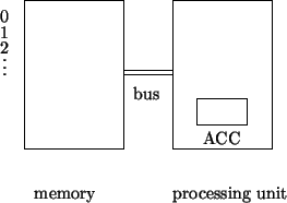
The memory is a set of labelled (i.e. numbered) locations which can hold information, such as numbers. The labels are known as addresses.

The bus is a bidirectional communications path, transmitting both addresses and numbers. (In practice, there may be several buses.)

The processing unit (usually referred to as the central processing unit, or CPU) can:

• copy information from one or more memory locations,
• process it (e.g. modify the copies by adding them together), and
• copy it back into either the same, or different, memory locations.

Therefore, there is usually a small amount of memory inside the CPU, to hold copies of information from the main memory and the results of computations. This is often in the form of registers, each of which can hold a single number. In MU0, there is a single register known as the Accumulator or ACC. (Intel use AX instead of ACC).

What the CPU actually does is controlled by a set of sequentially executed instructions, known as a program.

e.g. suppose that our example computer can perform the following actions:

LDA	x	copies the contents of location x to the ACC
ADD	y	adds a copy of the contents of location y to the ACC
STO	z	copies the contents of the ACC to location z
STP		stops the computer

MU0 instructions can only refer to memory locations and not directly to numbers. If we wanted to add one to a number, we would have to store the value 1 in a memory location (e.g. 12) and ADD 12.

These instructions are enough to add some numbers together and save the total e.g. we could use it in a cash till, to add the cost of all the individual items together to give the total cost:

Add an item price of #1.09 to a running total of #15.34

First we have to decide on the representation of prices inside the computer. A simple story is that #1.09 is represented by 109 and #15.34 by 1534. (We are ignoring problems such as the number base, the maximum number we can represent, and negative numbers - see CS1031.)

Now, suppose we somehow have the running total held in location 10 and the item price in location 11 (how this might be achieved is explained in CS1031):

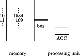
we could use the program:

LDA	10
ADD	11
STO	10
STP

then, if we set the computer to go through these instructions in sequence, it will:

• copy 1534 from location 10 and remember it in the ACC
• add 109, copied from location 11, to give 1643 in the ACC
• copy 1643 from the ACC back into location 10
• stop the program

and we end up with the answer, 1643 representing #16.43, in memory location 10 where we keep the running total, (and with a copy in the ACC) and the computer halted.

If we want to process more than one item, we somehow have to repeat this program, so we need to explore how the sequence of instructions can be controlled:

Stored programs and Program Counter

The list of instructions is clearly a vital part of the computational process and following it automatically is an essential part of the operation of a computer.

All practical digital computers use their memory to hold instructions as well as data (i.e. numbers or any other information that the program is working on) - thus "stored program". Computers have a Program Counter (PC) in the CPU which contains the address of the memory location containing the next instruction to be obeyed (executed). (Intel calls this the Instruction Pointer or IP.)

To be stored in memory locations, instructions have to be represented by numbers. The way in which an operation (encoded as a small integer e.g. LDA=0, STO=1, ADD=2) and a location are represented by a single number is similar to the way in which both pounds and pence are squeezed into a single number in the example above. The details of this representation are explained in the lab script, and can be seen using the simulator.

At the start of the program described above, the picture is now something like:

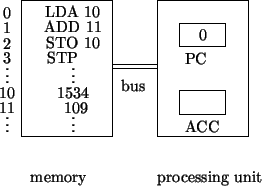
The computation starts with the PC set pointing to the address of the first instruction, in this case 0 (an arbitrary choice, as used in the MU0 simulator). The computation proceeds by executing the instruction pointed to by the PC and incrementing the PC by one. When the STP instruction is reached this process is halted.

Decision making

With linear lists of instructions, we can do limited things. Most of the power of computers comes from the power to change between different sequences of instructions as a result of tests on the stored information.

JMP, JNE & JGE, known collectively as jump instructions, allow us to change from one sequence of instructions to another. The second part of each jump instruction is the address of the start of the next sequence of instructions.
JMP is known as an unconditional jump, as it always causes a change, whereas JNE and JGE are known as conditional jumps, as they may or may not cause a change, depending on the current value in ACC: JNE causes a change only if the value is Not Equal to zero, and JGE if the value is Greater than or Equal to zero.

Suppose, in our cash till example, each new item price was magically put into memory location 11, and this was to be added to the running total until the item price was zero:

	LDA	zero	initialise total
	STO	10
again:	LDA	11
	JNE	more	if item non-zero then
	STP
more:	ADD	10	add non-zero item to total
	STO	10
	JMP	again	and try again
zero:	0

Notes:

• We need to initialise the running total to 0.
• I am using both explicit locations (10 and 11) and named locations (again, more and zero). An assembler will translate names to explicit location numbers as it converts the program into the representation stored in memory. In fact, it is normally preferable to use named locations all the time when writing programs.
• I have swapped the order of copying the contents of memory locations 10 and 11 to add them, to simplify the program. However, x+y == y+x, or else there is something seriously wrong!
• Very few real programs have their data magically appear in certain memory locations, but anything more realistic is beyond the capacity of this very simple computer! Real instruction sets for real computers will be covered in more detail in CS1031 and CS2042.